Stabilization Strategies for Nonlinear Static Abaqus Models
A common problem in nonlinear static Abaqus analyses is the presence of instabilities leading to non-convergence. Instabilities are often subtle and easily missed, leaving the analyst largely unaware of why the simulation failed and what to correct to get to a converged solution.
So, it is perhaps not surprising that Abaqus users often default to running simulations using automatic stabilization associated with the step definition (also known as static stabilization) to troubleshoot problematic models. However, automatic stabilization is not intended to be used as a one-size-fits-all tool to solve instabilities. In fact, when used inappropriately, it can produce unrealistic results that could lead to costly product failures.
To help analysts obtain a converged solution that is accurate, this blog will explain instabilities and suitable solving methods, focusing on when and how to use popular stabilization techniques in Abaqus/Standard to overcome them.
Typical warnings for non-convergence in Abaqus output files:

Figure 1
Understanding & Overcoming Instabilities
There are many ways to overcome instabilities to facilitate convergence, but it is essential to understand the main sources of instabilities and how they lead to non-convergence. Let's begin by understanding some possible sources of nonlinearity:
- Geometry – A geometrically nonlinear analysis is one in which the structure's stiffness changes as it deforms. Some examples are:
- Large deflections and deformations, large rotations, structural instabilities (buckling), etc.
- Material – Material nonlinearity is caused by the dependence of the stress on the current strain. Some common effects are:
- Nonlinear elasticity, metal plasticity, cracking, crushing, necking, etc.
- Boundary (Contact) – Discontinuous stiffness change due to the nature of contact, which is defined by normal and tangential behaviors. Normal contact is either established or not, and tangential is either open, slipping, or sticking. These are always a sudden change in stiffness and are thus classified as Discontinuous.
Note that a consistent theme to these instabilities is a change in stiffness – the greater the change in stiffness, the greater the risk of non-convergence.
To understand why this is important, return to the fundamentals of what makes a problem static or dynamic. Put simply, the difference is the presence of inertial effects:
Dynamic Equilibrium
| P – I = ma | ||
| m = Mass Matrix | P = External Forces | I = Internal Forces |
| a = Acceleration | v = Velocity | u = Displacement |
Static Equilibrium
When inertial forces are small (ma –> 0), the equation reduces to the static form of equilibrium.
| P – I = 0 | ||
| I = Cv + Ku | ||
| C = Damping | K = Stiffness | K = EMa |
| E = Elastic Modulus | Ma = Moment of Area |
For a static analysis, notice that there is no inertia and that the solution is dominated by the components associated with damping and stiffness.
Thus, with no damping and sudden changes in the stiffness when the structure starts to buckle/bend or the material softens, zero stiffness between objects, such as contact gaps and unconstrained rigid body motion, makes it difficult for the static solver to converge to a solution.
Therefore, the absence of inherent damping, coupled with abrupt shifts in stiffness (due to phenomena like buckling, bending, or material softening) or even the total absence of stiffness in situations like contact gaps or free body motion, often makes it challenging for the static solver to reach a converged solution.
There are three commonly considered options to overcome this:
- An implicit dynamic (quasi-static) procedure in Abaqus/Standard
- A dynamic procedure in Abaqus/Explicit
- A static procedure with stabilization using Abaqus/Standard
Since the topic of this article is static nonlinear problems, we turn our attention to the third option: employing stabilization within the Abaqus/Standard solver.
As mentioned at the beginning of this blog article, because of its widespread overuse and potential negative consequences, we must be careful about when static stabilization is applied.
Static stabilization is used primarily to overcome convergence issues triggered by global instabilities or phenomena causing changes in the global stiffness, such as buckling of the entire structure, material softening, or unconstrained rigid body motion. This option is activated while defining the step details in a static procedure. To use it, you could use one of the options available, such as specifying a damping factor or a dissipated energy fraction.
- If you specify a damping factor, a constant value will be used throughout the step. This value is usually chosen based on trial and error or prior experience.
- If you choose to use dissipated energy fraction – the ratio of stabilization energy (ALLSD) to total internal energy (ALLIE) of the model, Abaqus will adjust the damping factor, maintaining the ratio below the specified value. The default value is 2.0e-4. You can also control adaptive behavior by setting a tolerance value. If the ratio exceeds it, Abaqus will automatically adjust the damping factor in subsequent increments. If the tolerance is set to 0, a constant damping factor (based on the initial energy fraction) will be used.
The choice of these stabilization options and their input must be made with caution and understanding. The energy dissipation in the model must be monitored to ensure it is within reasonable limits. We do this by monitoring history output quantities – Stabilization energy (ALLSD) and internal energy (ALLIE) of the model. This is to ensure that the addition of stabilization does not significantly influence the physical behavior being changed.
The Abaqus manual advises keeping ALLSD below 5% of all ALLIE. Minimizing this stabilization energy percentage can help move towards physical behavior. The adaptive stabilization option, which adjusts the damping factor based on convergence behavior, is a useful option to consider, ensuring that the adaptive damping values used do not cause the stabilization energies to exceed the strain energy values.
Building upon our understanding of when and how to use step-based static stabilization, we will now turn our attention to another common stabilization option in Abaqus/Standard: the Contact Controls Stabilize feature used with Contact Pairs.
For more details, reference Figure 2 below.
Stabilization Applied to Contact Pairs
We discussed earlier that contact is a highly nonlinear form of nonlinearity, where the state of interaction between regions can keep changing – either sticking, slipping, or opening up.
In scenarios where bodies are approaching to establish contact, convergence can be problematic prior to full engagement due to the inability to establish equilibrium.
Consider a simulation where a force is applied to a spherical indenter to move it towards a second body. Initially, while a gap exists between the two, the indenter will behave as a rigid body. This occurs because without contact, there's no opposing force or boundary to generate a reaction, preventing static equilibrium from being achieved. While the mechanism for stabilization is the addition of viscous damping, it would be helpful to think of adding stabilization in this scenario as having an effect similar to temporary weak springs at the contact interface. An opposing reaction force would develop and contribute to the attainment of static equilibrium or convergence.
Another scenario could be where there is full contact between the objects, but there is relative motion between the two contact surfaces. This change in state can cause what we could imagine as numerical shocks. Stabilization within the contact pair framework can help dampen these shocks and help smoothen the process of achieving numerical convergence and reduce instability.
Here are a few tips for applying stabilization efficiently to contact pairs:
- Apply stabilization to the relevant Contact Pair – Since a common source of instabilities in models stems from Boundary (Contact) problems, it is best to target the contact pairs with need for stabilization to facilitate establishing initial contact. This helps to minimize the amount of stabilization used and thus reduce the potential for error.
- Stabilization is applied to the contact pair at the beginning of the step, and users can choose to ramp its value down to zero (or a very small value) by the step's end. This is best suited to contact pairs with a gap between them at the beginning of the step (unconstrained rigid body motion, DOF numerical singularity, unconnected regions). To do this in Abaqus/CAE, create a Contact Controls definition with Automatic Stabilization, and on the Contact Pair, select the drop-down box for your Contact Control as shown in Figure 2 below.

Figure 2
- Stabilization is applied to the contact pair at the beginning of the step, and users can choose to ramp its value down to zero (or a very small value) by the step's end. This is best suited to contact pairs with a gap between them at the beginning of the step (unconstrained rigid body motion, DOF numerical singularity, unconnected regions). To do this in Abaqus/CAE, create a Contact Controls definition with Automatic Stabilization, and on the Contact Pair, select the drop-down box for your Contact Control as shown in Figure 2 below.
- Check the Energies – A good practice is to always check the stabilization energy (ALLSD) against the internal energy (ALLIE) of the model. The recommendation is to keep ALLSD to less than 5% of ALLIE. However, in practice, you could try to reduce this to a much lesser value (e.g., 1% or even less) and still have a converged model, so it's good to try out a few iterations by decreasing stabilization.
- Remember, stabilization is artificial, and the greater the amount present, the greater the potential for error in the overall solution.
- Too much stabilization can be a bad thing, too. It can cause non-physical behavior or can cause non-convergence.
- Figure 3 shows an example - a history plot of energies, where excessive stabilization is evident from the stabilization energy curve (ALLSD).
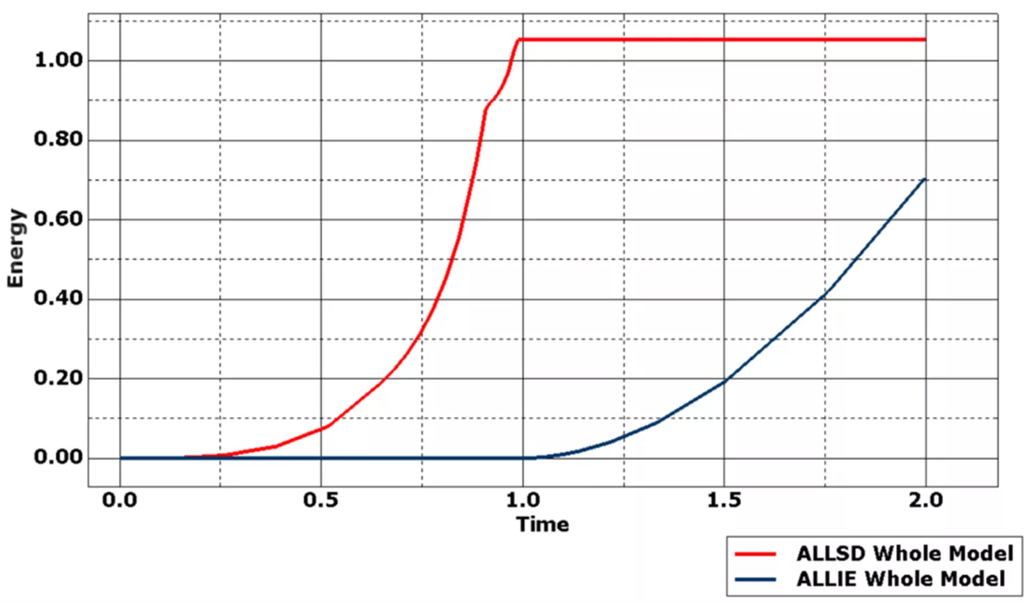
Figure 3
- Add a Step for Establishing Contact – Another way to reduce the error created by stabilization and facilitate convergence in models with contact pairs is to split the load step into two load steps. In the first step, apply stabilization, but apply a small fraction (1-10%) of the maximum load. That way, contact can be established, negating the need for stabilization in the subsequent step in which the load can be ramped up to the maximum load. You can see in Figure 3 that the stabilization energy increases in step 1 but remains constant in step 2. In Abaqus/CAE, you can set this up as follows:

Figure 4
An Illustrative Example of Results from Applied Recommendations
To understand these concepts better, we'll apply these recommendations to a simple analysis model (that we’ll call model ‘A’). This model initially encounters convergence issues or fails to solve. The warnings generated in its message file are shown in Figure 1. We then split the load applied across two steps and vary the automatic stabilization factor to try to bring down the stabilization energy quantity, and these generate variants that we call model ‘B’ and model ‘C’.
To track the impact of these recommendations and variations in stabilization, we will record the essential input parameters and the observed output data in the table shown below:
| Steps | Load | Automatic Stabilization Factor | ALLSD/ALLIE (%) | Peak Stress | Peak Stress (%) | |
| A | 1 | Step 1 = 100% | 1 | 13,725% | 80.25 MPa | 97% |
| B | 2 | Step 1 = 1% Step 2 = 1-100% |
1E-2 | 149% | 82.59 MPa | 99.9% |
| C | 2 | Step 1 = 1% Step 2 = 1-100% |
1E-8 | 0.27% | 82.64 MPa | 100% |
You can observe that the analysis in row A has a single step where the full load is applied and automatic stabilization with a factor of 1 is active on the contact pair. Checking the ratio of ALLSD/ALLIE in the results, we observe a value of 13,725%, clearly violating the 5% recommendation.
Model ‘B’ has a second step added, with the applied load being a 1% fraction of the total load in the first step and increased to 100% in the second step. The Stabilization Factor is reduced to 1E-2 and applied only in the first step. Checking the ratio of ALLSD/ALLIE, we see that it is 149%, less than the previous analysis but still violating the 5% recommendation.
We make further changes in Model ‘C’ - the stabilization factor is reduced from 1E-2 to 1E-8, and as a result, we can see that the ALLSD/ALLIE ratio is now at 0.27%, clearly less than the 5% recommendation. Since Model ‘C’ has the lowest ratio of ALLSD/ALLIE, we expect its simulated behavior to be closer to the ‘real world’ compared to the previous two.
It's also worth noting that stabilization introduces a damping-like effect, resisting relative incremental motion between the contacting surfaces. Even in a 'static' analysis, the solver works through small incremental displacements over small amounts of pseudo-time (since time is a non-physical quantity in a static analysis). Pseudo-time helps track the solver's incremental progress. Therefore, the larger the relative incremental displacements are during these pseudo-time increments (effectively acting like a higher relative velocity for the stabilization algorithm), the larger the artificial damping force applied for that increment will be. This means that if you run the same model a few times but change some characteristics, like the friction between the contact surfaces, you might see different levels of stabilization being automatically applied, leading to inconsistent effects on results like peak stress.
In conclusion, stabilization is a very powerful tool for achieving convergence in nonlinear static problems. Apply stabilization responsibly to ensure the results are as 'realistic' as possible.
Ready to get started with Abaqus? Read our Abaqus buying guide or contact us to talk to GoEngineer's simulation experts to find the right tool for you! If you’re not ready to use Abaqus yourself, you can still take full advantage of its benefits through FEA consulting from GoEngineer.
Editor's Note: This article was originally published in June 2021 and has been updated for accuracy and comprehensiveness.
Related Articles
Abaqus Meshing Tips for Accurate Stress Results
7 Abaqus/CAE Tips for New Users
Enhancing EV Connector Design Using Abaqus FEA
FEA Materials Are Make-or-Break: Introducing the 3DEXPERIENCE Material Calibration App
Structural FEA for Beginners: 5 Stages of Simulation-Driven Design

About Vikram Radhakrishnan
Vikram is part of the Simulation team at GoEngineer, where he helps engineers leverage Dassault Systèmes technologies to solve real-world challenges. With nearly two decades of experience across Aerospace, Automotive, Marine, Energy, and Manufacturing, he brings deep expertise in structural mechanics, multiphysics, and engineering automation. Outside of work, you’ll likely find him at the table tennis table, sharpening his backhand.
Get our wide array of technical resources delivered right to your inbox.
Unsubscribe at any time.