Abaqus Meshing Tips for Accurate Stress Results

Reliable stress results are crucial for making informed engineering decisions, ensuring safety, and optimizing designs. When running a simulation, it’s essential that the results align with real-world observations, despite the assumptions and approximations present in any analysis. Achieving accuracy in Abaqus isn’t just about building your model and clicking the “run” button.

Careful modeling and analysis setup are necessary to avoid errors and misleading results. A sufficiently refined mesh with appropriate element choices is the best way to balance efficiency and accuracy in analysis results. This blog explores key meshing techniques to improve the accuracy and reliability of stress results in Abaqus.

Element Type Selection

Choosing the right element type is the first critical step in mesh generation. Should you use solid (3D), shell (2D), or beam (1D) elements—or a combination?

With accuracy as the goal, it may seem that solid elements are the obvious choice. After all, the real world is three-dimensional; shouldn’t you use three-dimensional elements to reflect that, instead of simplifications?

In reality, testing shows that shell or beam elements, when appropriately chosen, provide accurate results while saving computational resources. In general:

• Shell meshing is useful for thin bodies with a uniform thickness (sheet metal, etc.)
• Beam meshing is best suited for – you guessed it – beams (and trusses), particularly when the beam’s length is at least ten times its cross-sectional diameter.

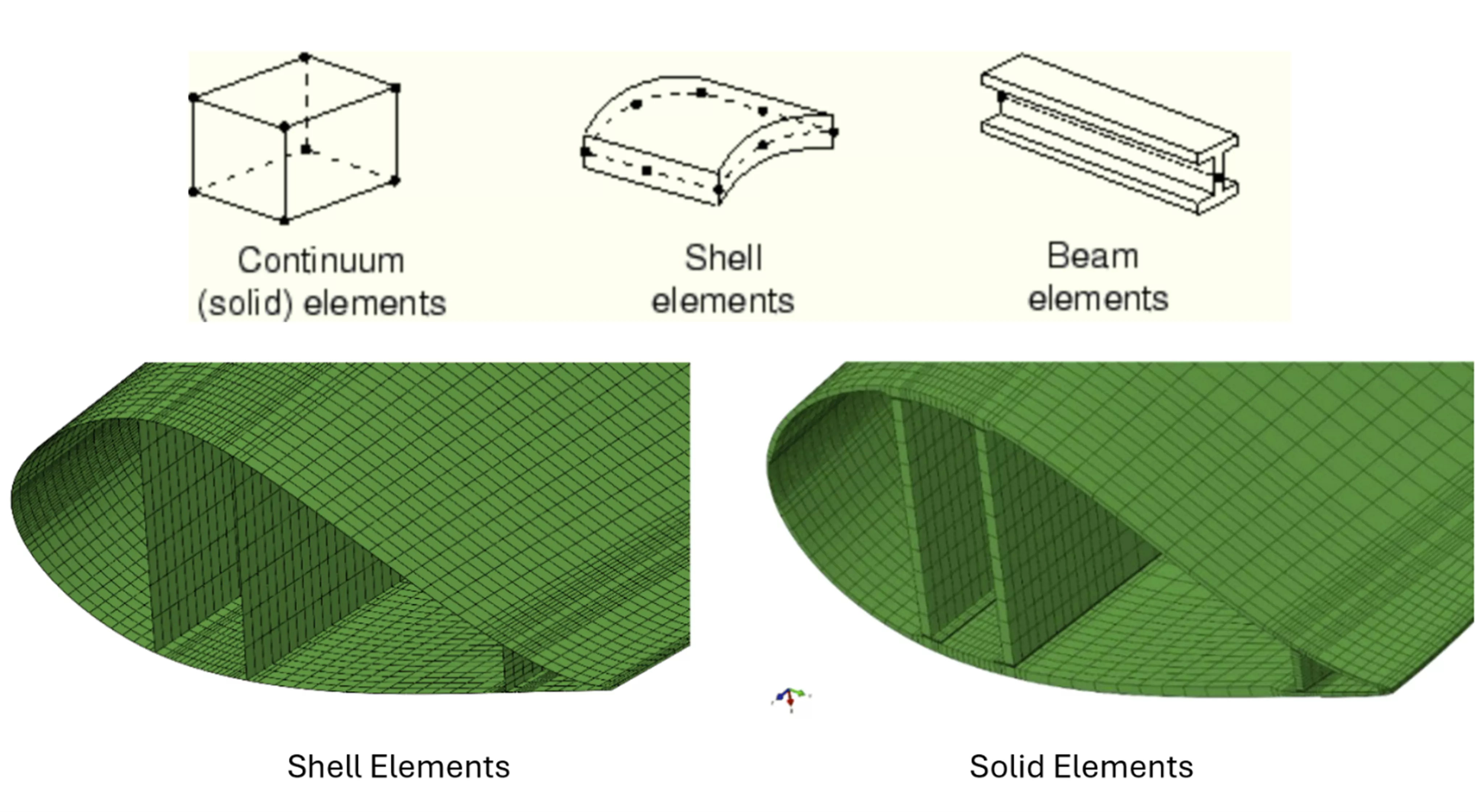
Figure 1: Example of solid, shell, and beam elements

Suppose you need to calculate the deflection at the end of a 1.5 m cantilever beam (square cross section 0.05 m x 0.05 m) under a uniform 200 N/m load:

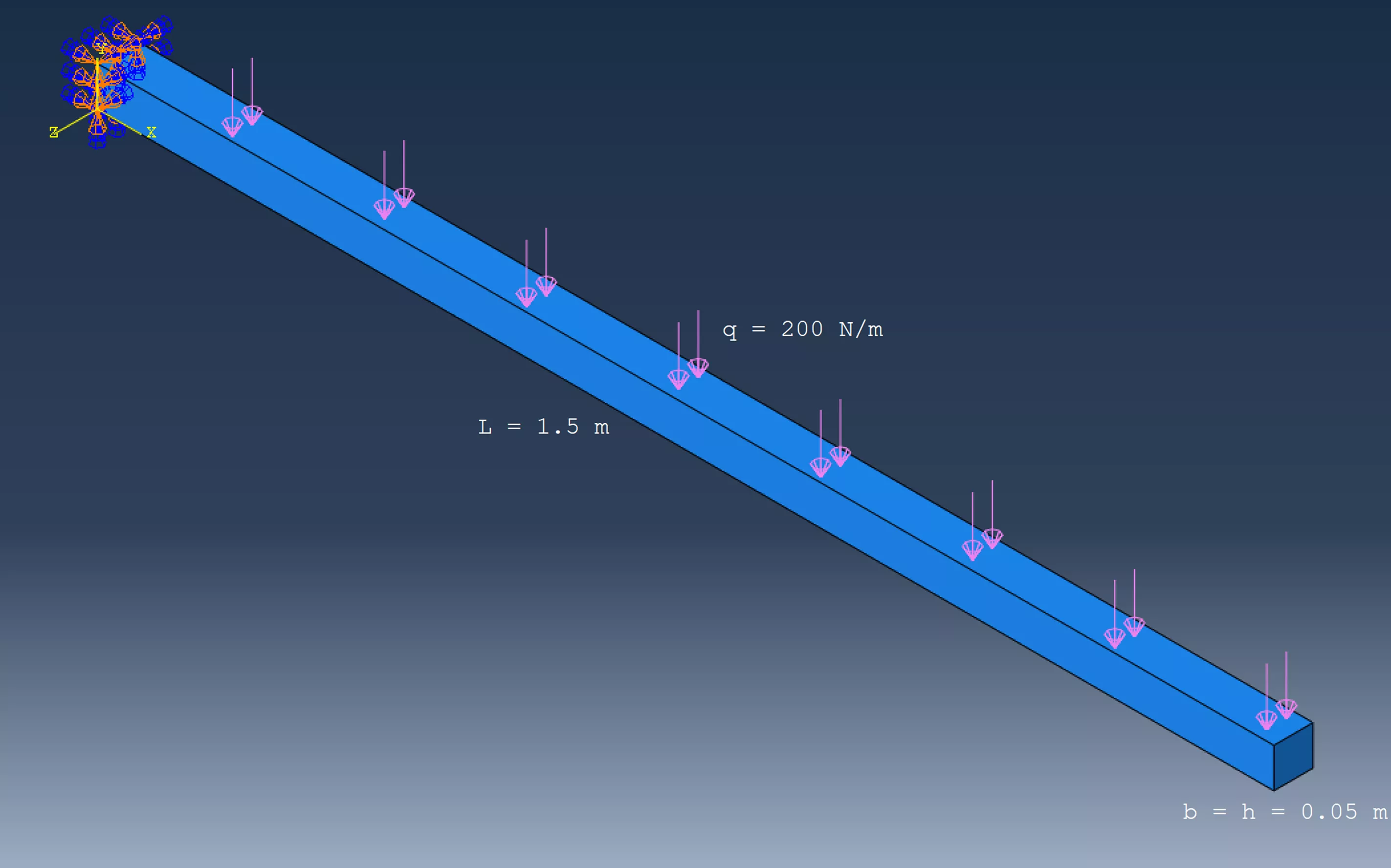
Figure 2: Cantilever beam problem setup

Let's do the math...

Maximum deflection (δ) = (qL⁴)/(8EI)

• q = force applied = 200 N/m
• L = beam length = 1.5 m
• E = elastic modulus = 50 GPa
• I = moment of inertia = (1/12)b⁴ = (1/12)(0.05)⁴ = 5.208333e–7 m⁴

δ = (200 * 1.5⁴) / (8 * 50e9 * 5.208333e–7)

  = 0.004860 m

  = 4.860 mm

The math tells us the maximum deflection is 4.860 mm. If I model this in Abaqus and mesh it with solid elements, here are the results at various mesh sizes:

Solid Element Size	Number of Elements	Maximum Deflection	Error from Calculated
0.05 m	30	5.880 mm	20.99%
0.025 m	240	4.774 mm	1.77%
0.01 m	3,750	4.829 mm	0.64%
0.005 m	30,000	4.846 mm	0.29%

Figure 3: Table of results when using solid elements

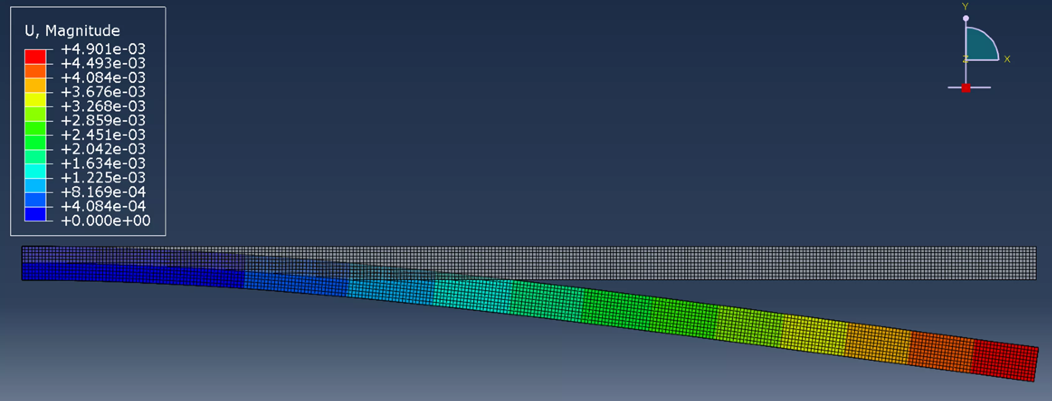
Figure 4: Beam deflection results

If this same model is meshed with beam elements, here are the results:

Beam Element Size	Number of Elements	Maximum Deflection	Error from Calculated
0.05 m	30	4.867 mm	0.14%
0.025 m	60	4.866 mm	0.12%
0.01 m	150	4.866 mm	0.12%
0.005 m	300	4.866 mm	0.12%

Figure 5: Table of results when using beam elements

So, while solid elements are three-dimensional and therefore the closest representation of the real world, it takes a very fine mesh to approach the calculated answer - around 3,000 elements are needed to get <1% error. Compare this to the beam results: with just 30 elements, my answer is already within 0.14% of the calculated value.

A similar idea can be applied to shell meshing. When appropriate, shell meshing can be at least as accurate as solid meshing while saving valuable computational resources. Always consider the shapes of the bodies being analyzed and choose an appropriate element type.

Element Quality and Formulation/Integration

Once the element type has been selected, the next choice is between first-order (linear) and second-order (quadratic) elements, which define the resolution and quality of each element, followed by the type of element integration.

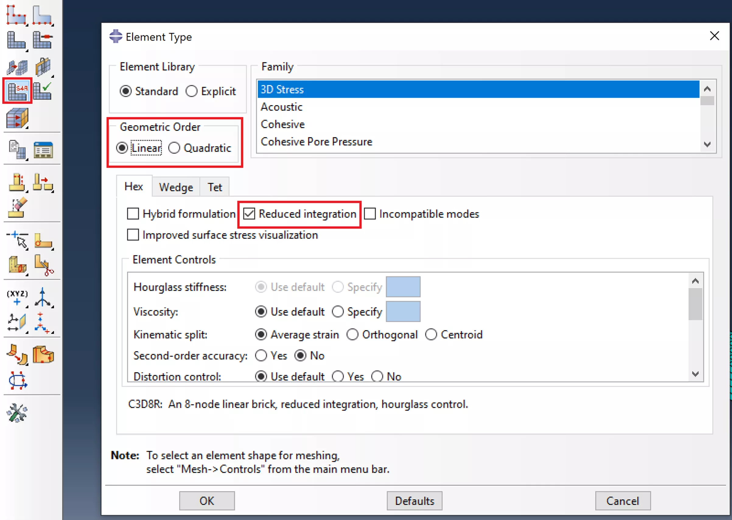
Figure 6: "Assign Element Type" dialog, where integration and order are chosen

First-Order vs Second-Order Elements in FEA

First-order elements have nodes at each corner, while second-order elements have additional nodes at the midpoint of each side.

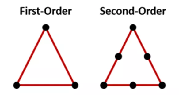
Figure 7: The difference between first and second order elements

The additional nodes in second-order elements introduce additional degrees of freedom, causing less stiffness and more accurate deflection than stiffer first-order elements. However, higher quality elements come with a higher computational cost and therefore longer solve times. There are some scenarios, particularly high-speed dynamic situations such as a car crash or a drop test, in which first-order elements are the more stable choice.

Another key consideration is element formulation and integration. There are the following integration options:

• Full integration calculates displacement at all integration points, known as “Gauss points,” of each element (e.g., C3D8 elements).
• Reduced integration (such as C3D8R elements) calculates displacement based on one central Gauss point for each element.
• Selective reduced integration (such as C3D8I) is a combination of both: elements in areas of concern (e.g., high shear or volumetric strain) will be fully integrated at all Gauss points, while elements elsewhere will use reduced integration.

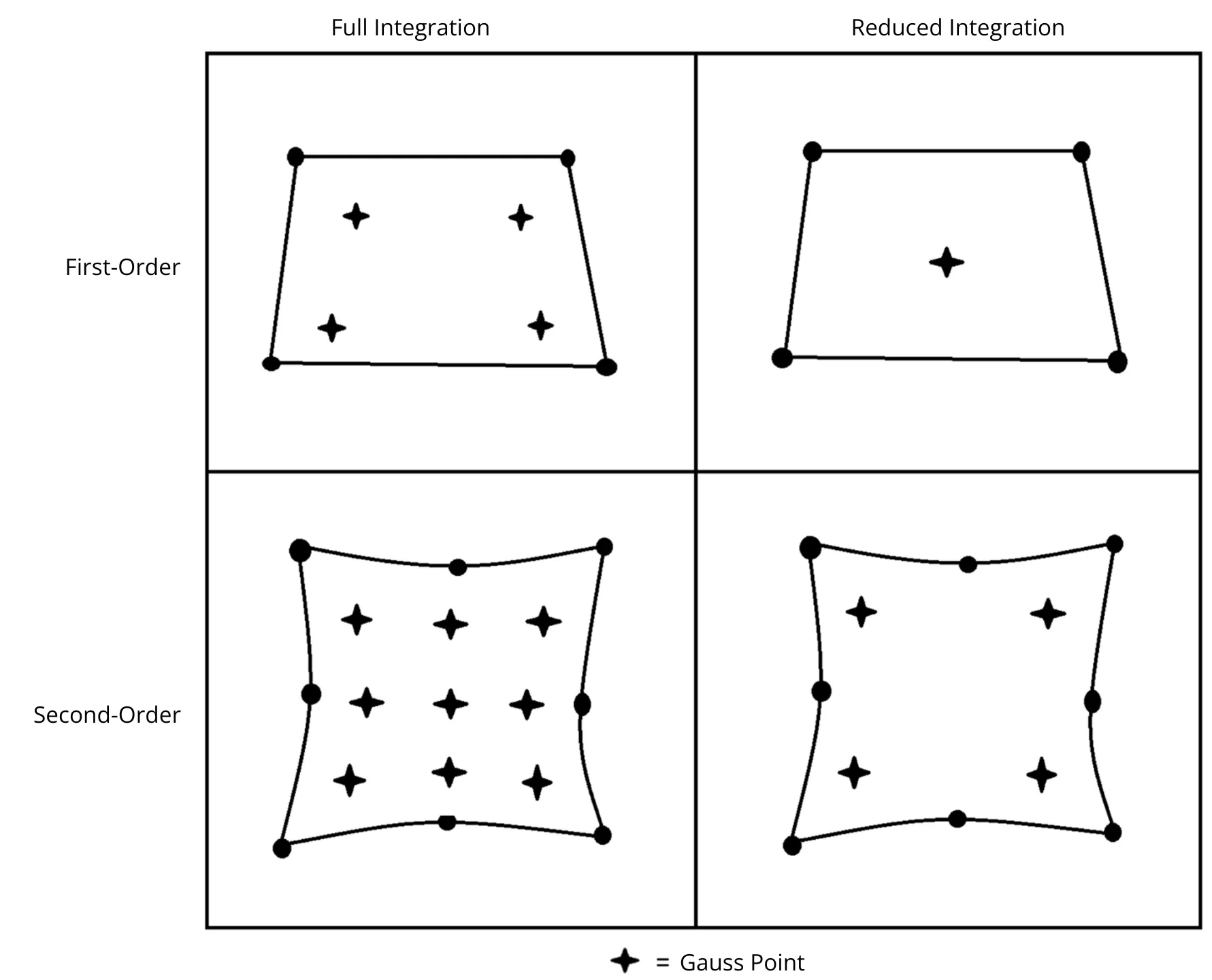
Figure 8: The difference in element integration types

As with most choices to be made when setting up a model for analysis, each option comes with advantages and disadvantages that must be balanced to maximize accuracy and efficiency:

Integration Type	Advantages	Disadvanates
Full	Most accurate stress results Reduces risk of hourglass modes	Computationally expensive Susceptible to locking (artificially high stiffness) with bending or nearly incompressible problems
Reduced	Faster computations Reduces shear and volumetric locking	Prone to hourglass modes (artificial zero-energy modes) Less accurate in stress calculations, especially in bending-dominated problems
Selective Reduced	Balances accuracy and efficiency Reduces locking while maintaining accuracy	Slightly more computationally expensive than reduced integration

Figure 9: Pros and cons list for full, reduced, and selective reduced integration

Returning to my cantilever beam example, I meshed and solved the study with four different element formulations: First-Order/Full Integration, Second-Order/Full Integration, First-Order/Reduced Integration, and Second-Order/Reduced Integration. Here is a table of the results:

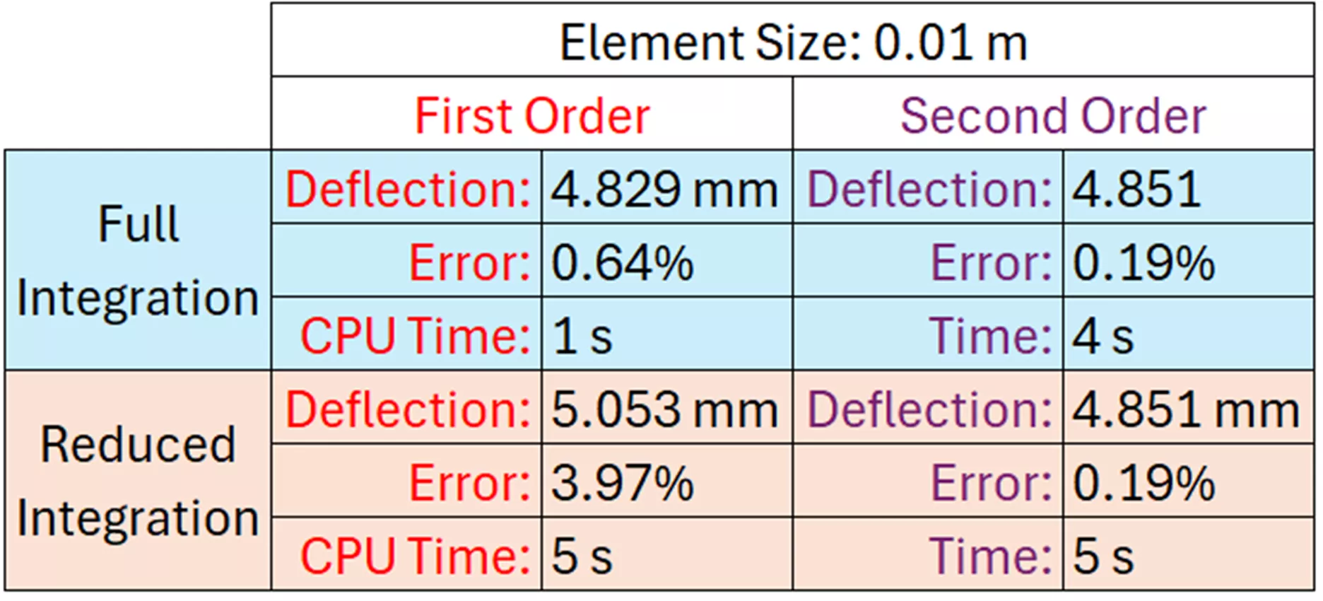
Figure 10: Results comparing element order and integration in cantilever beam problem

For this type of simple problem, it is evident that solve time is not much of an issue. However, there is a notable difference in accuracy depending on the formulation chosen. The best option is clearly Second-Order/Full Integration, which gives us results very close to the calculated answer of 4.860 mm, without the need for further mesh refinement.

The following table lists a variety of analysis types with their recommended element quality and formulation choices:

Problem Type	Recommended Element Type
Bending (no contact)	Second-Order Full Integration
Stress Concentration	Second-Order Full Integration
Natural Frequency (linear dynamics)	Second-Order Full Integration
Complicated Model Geometry (linear material, no contact)	Second-Order Hexahedral (if not distorted), Second-Order Tetrahedral (if meshing difficulties)
Complicated Model Geometry (nonlinear problem or contact)	First-Order Hexahedral (if not distorted), Second-Order Tetrahedral (if meshing difficulties)
Nearly Incompressible (v > 0.475)	First-Order, or Second-Order Reduced Integration
Completely Incompressible (v = 0.5)	Hybrid (first-order if large deformations expected)
Bulk Metal Forming (high mesh distortion)	First-Order Reduced Integration
Contact With Bending	First-Order Reduced Integration
Nonlinear Dynamic (impact)	First-Order Full Integration
Contact Between Deformable Bodies	First-Order Full Integration

Figure 11: Recommended element types for various problem types

More: Element formulation and integration - SIMULIA User Assistance 2024

Mesh Quality Checks

When the type of mesh is selected, the mesh is ready to be generated. Then, you need to verify its quality. A distorted, skewed, excessively angled mesh can cause calculation errors, so you need to find and minimize these issues.

You can access Abaqus’ mesh verification tool by switching to the Mesh module and going to Mesh > Verify. This tool detects and highlights elements in your mesh that fail to meet criteria for corner angles, aspect ratio, edge length, and more. These criteria can be user-specified, but the default values are typically sufficient.

Any problematic areas you find with this tool can be resolved with further mesh refinement via global or local mesh controls. Smaller element sizes will help reduce distortion and aspect ratios.

More: Verifying your mesh - SIMULIA User Assistance 2024

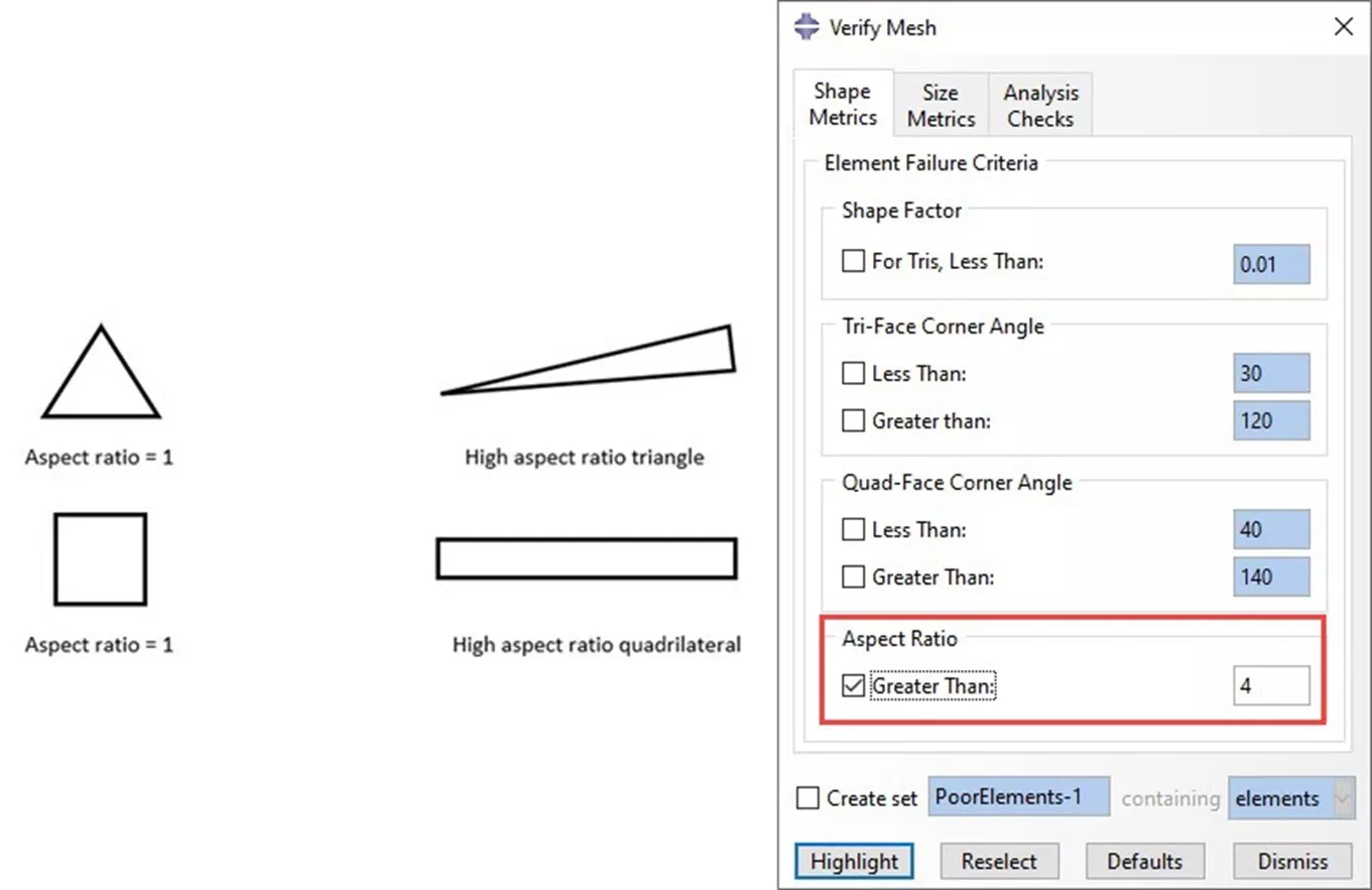
Figure 12: Element aspect ratios and how to verify mesh quality

Mesh Sensitivity Analysis

Even after creating and verifying a high-quality mesh, blindly trusting results without checking for convergence is risky. A mesh sensitivity analysis involves running the simulation with progressively refined meshes to see when the results stabilize.

For example, let’s return to the cantilever beam example presented earlier. You can see that mesh refinement was necessary to approach the theoretical answer of 4.860 mm. However, at a certain point, additional refinement does not significantly improve results and only slows down the calculation.

Solid Element Size	Number of Elements	Maximum Deflection	Error from Calculated
0.05 m	30	5.880 mm	20.99%
0.025 m	240	4.774 mm	1.77%
0.01 m	3,750	4.829 mm	0.64%
0.005 m	30,000	4.846 mm	0.29%
0.0025 m	240,000	4.851 mm	0.19%

Figure 13: Results at decreasing element sizes

If you start with a coarse mesh, then refine until results converge, you can be confident that your result is an accurate calculation of the problem we set up.

More: Design sensitivity analysis for cantilever beam - SIMULIA User Assistance 2024

However, there are a few more ways you can optimize your mesh to run as efficiently as possible, without sacrificing accuracy.

Submodeling, Adaptive Meshing, and Local Mesh Control

With a sufficiently refined mesh made of an appropriately chosen element type and formulation, we are well on our way to generating reliable results in Abaqus. But cranking up the mesh refinement and giving your computer all it can handle might not be the most efficient technique to find the answers you need from an analysis.

Submodeling

Submodeling is a technique used to focus mesh refinement on regions of interest without needing to refine the entire model’s mesh. This provides accurate results where needed without forcing your system to make unnecessarily precise calculations elsewhere.

When submodeling, you start with a coarse global mesh of the full model to capture overall structural behavior, which is saved as nodal results. You then run an analysis on a smaller region of the model (called a submodel) with a fine mesh, applying the displacement/stress boundary conditions inherited from the coarse global model.

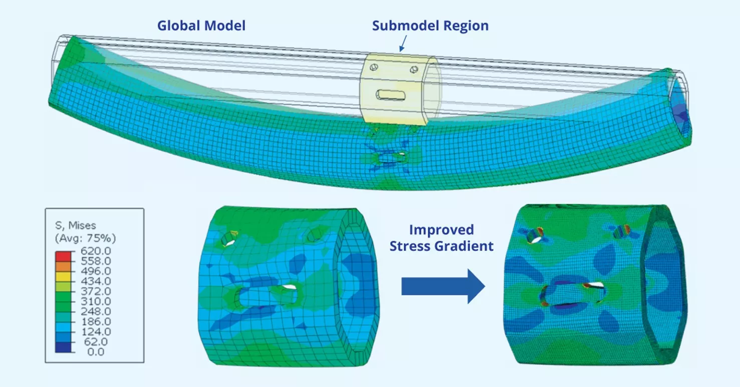
Figure 14: Submodeling technique 

This multi-step approach is a great way to handle large models containing smaller, more detailed areas of concern, without demanding excessive computational resources.

More: About Submodeling - SIMULIA User Assistance 2024

Adaptive Meshing

Adaptive Meshing applies a similar concept (fine mesh in areas that need it, coarse mesh elsewhere), but it works automatically during a solve. With adaptive meshing, Abaqus identifies regions where stress gradients are high and automatically refines the mesh in those specific regions. This helps with convergence and monitors the solve for errors without needing to manually analyze and update your mesh, and without needing an excessively refined global mesh.

More: About ALE Adaptive Meshing - SIMULIA User Assistance 2024

Local Mesh Controls

Beyond these options, your mesh can be manually refined however and wherever you like, with Local Mesh Controls. Local Mesh Controls allow you to input specific element sizes in specific areas as needed, while keeping the global mesh reasonably coarse. Rather than letting Abaqus make these changes automatically with Adaptive Meshing, some users prefer the full control offered by Local Mesh Controls.

More: Assigning mesh controls - SIMULIA User Assistance 2024

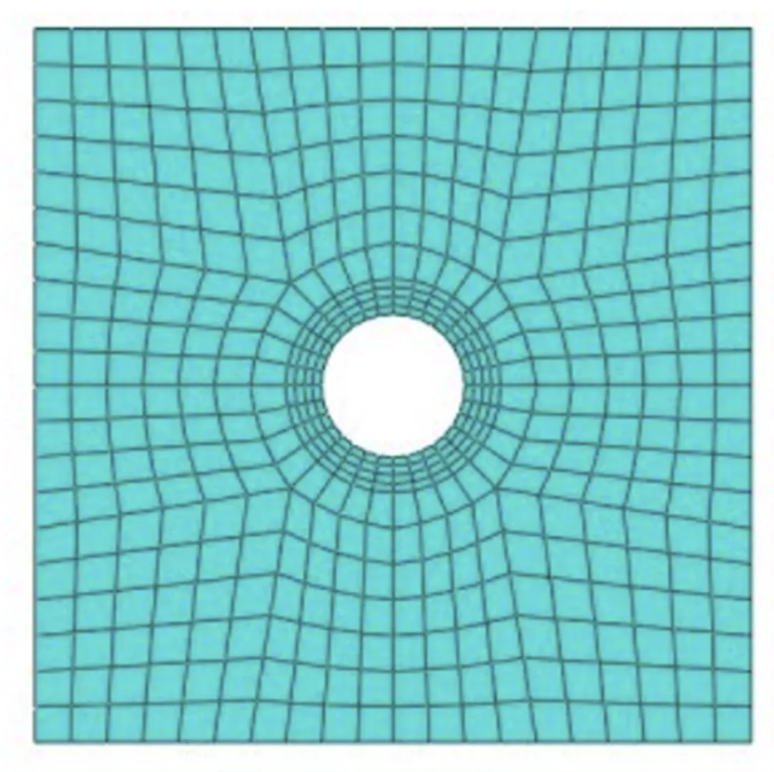
Figure 15: Body with coarse global mesh and fine local mesh control at area of interest

There are even more options to play with in Abaqus when it comes to element selection and meshing, and GoEngineer’s team can help you make sense of it all to create informative, accurate analyses. Visit our Application Mentoring Sessions page and book time with an expert.

Conclusion

Accurate stress results in Abaqus are essential for reliable engineering analysis, design improvements, and the prevention of costly errors. Thoughtful meshing decisions minimize calculation issues and unrealistic deformations. Refining your mesh, using appropriate element formulations, and validating your results through sensitivity studies helps ensure that your studies reflect real-world behavior.

By applying these best practices, you can improve the reliability of your models, leading to more confident design decisions and safer systems. A well-constructed simulation isn’t just about generating results; it’s about ensuring those results can be trusted.

Abaqus Training

Want to take your skills to the next level? Our course catalog contains 10+ online, instructor-led, or self-paced Abaqus training courses from introductory courses to advanced topics. View our course catalog for details.

I hope you found these Abaqus Meshing tips for accurate stress results helpful. Check out more tips and tricks below. Additionally, join the GoEngineer Community to participate in discussions, create forum posts, and answer questions from other Abaqus users. 

Related Articles

7 Abaqus/CAE Tips for New Users

Abaqus Solvers: Empowering Engineers in Every FEA Scenario

Understanding Abaqus General Contact

Abaqus - Modeling Arbitrary Shaped Beam Cross Sections

FEA Critical Speed Analysis & Rotor Dynamics

VIEW ALL ABAQUS ARTICLES