CST Studio Suite Hybrid Solver for System-Level Electromagnetic Analysis
Simulating electrically large and highly complex structures is a challenging task due to the high aspect ratio between the smallest details and the overall calculation domain. Analyzing these multi-scale problems can be time-consuming and can demand substantial computational resources if you use a single numerical method (brute force method).
A more efficient way to perform a system-level electromagnetic analysis is to divide the large problem into sub-domains. This allows the most suitable method to solve a particular sub-domain in the simulation, which leads to a faster analysis and, in turn, shortens the product development cycle. In CST Studio Suite, this approach is called the Hybrid Solver Task.
Figure 1(a) shows the simulation of a parabolic dish reflector antenna with a feed horn antenna. Instead of using a single solver (time domain solver) to mesh and analyze the full system—requiring a 3D discretization of free space between source and platform— you can use the Hybrid Solver Task. This method creates two simulation projects: one for the horn antenna and one for the reflector, which simulates sequentially.
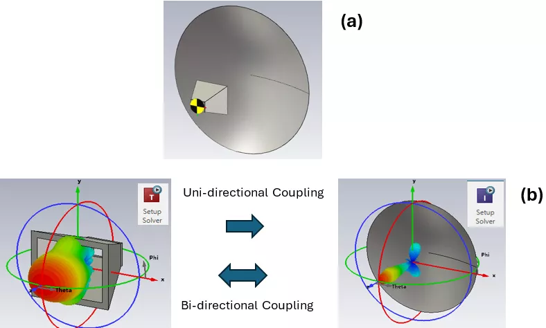
Figure 1: (a) Horn fed dish reflector (b) Horn antenna and reflector dish separated into 2 projects
A hybrid solver can be easily set up using the Hybrid Solver Task in the System Assembly and Modeling (SAM) interface.
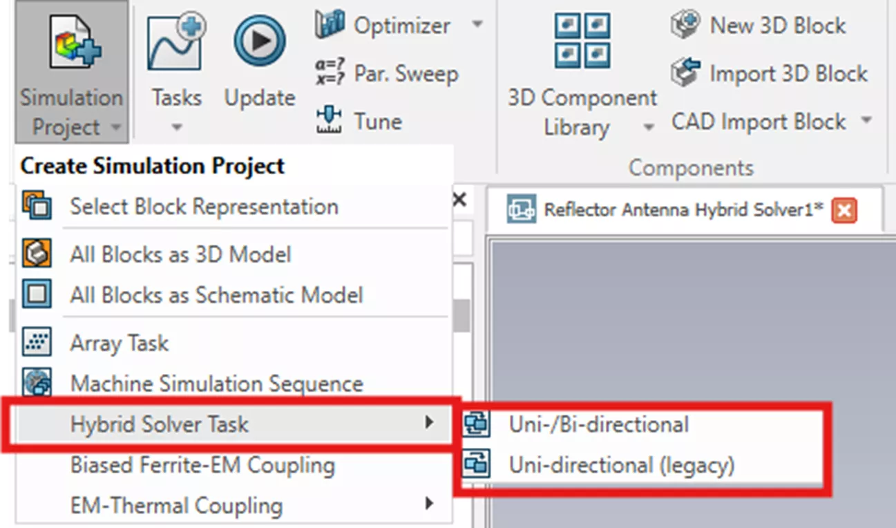
Figure 2: Hybrid Solver Task
There are two coupling methods (Figure 2) to choose when setting up the Hybrid Solver Task:
- Uni-directional: For setups where little or no field coupling between source and platform domains (i.e., loosely coupled systems). The sources are calculated first. The coupling data (near-field or far-field) will be from source domain to platform domain only.
- Bi-directional: Exchange coupling data iteratively between source and platform domains (i.e., tightly coupled systems).
Creating a simulation project (figure 4(a)) of a platform (reflector dish) and a source (feed horn antenna) as shown in figure 4(b) and figure 4(c) respectively, will allow you to assign the most appropriate solver to use in each project. In this case, Integral Equation Solver (I-solver) for the platform project and Time Domain Solver (T-Solver) for the source project are chosen. Depending on the location of the source relative to the overall system, both near-field source and far-field source can be used as excitation for the dish reflector.
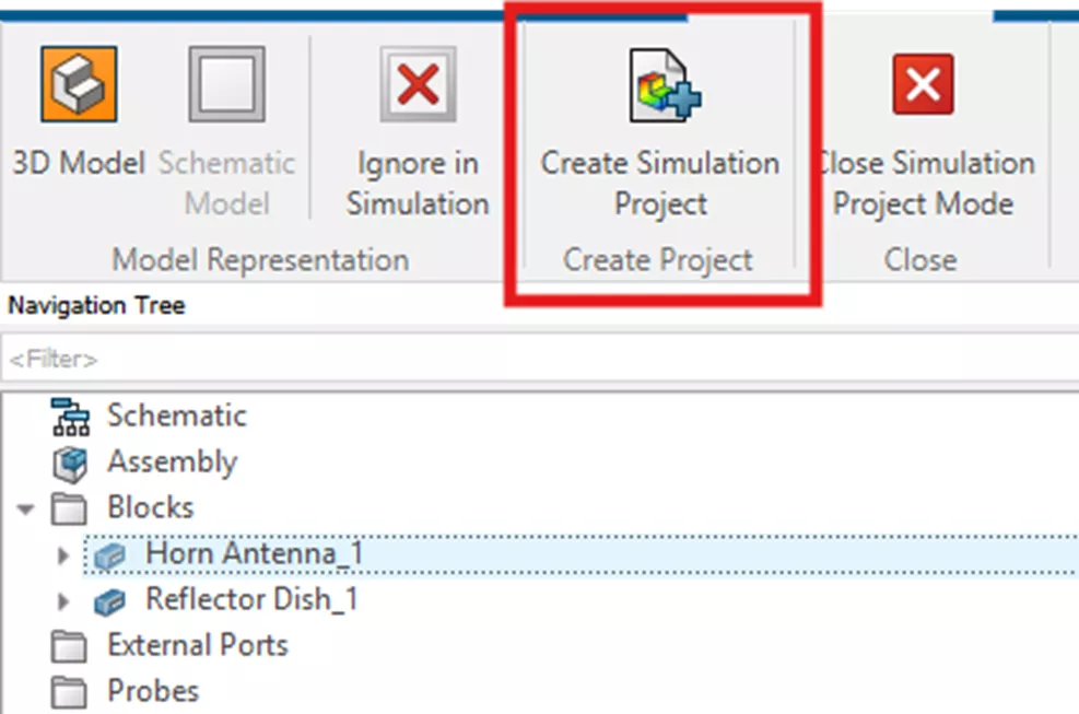
Figure 4 (a): Create Simulation Project
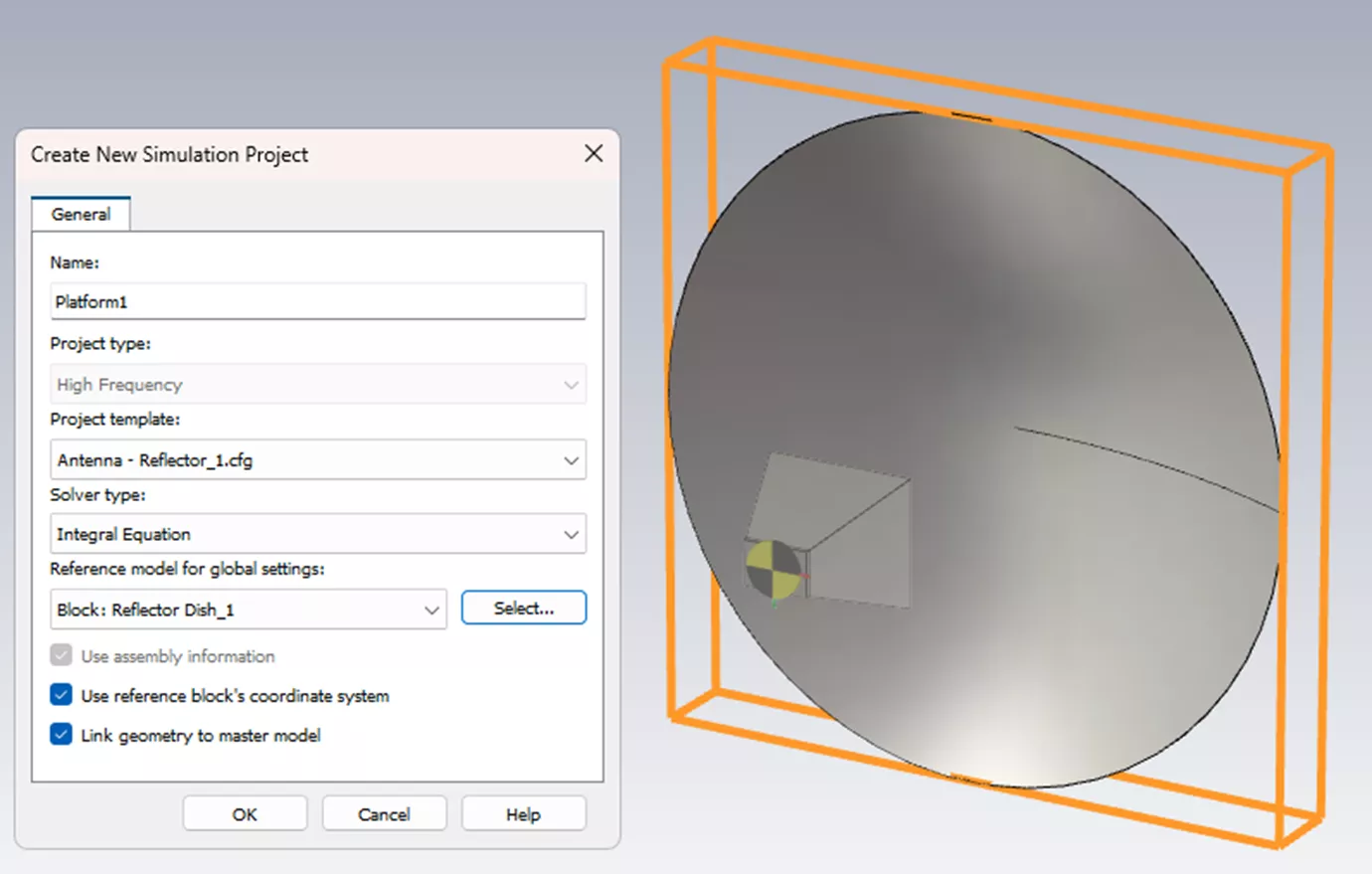
Figure 4 (b): Platform project
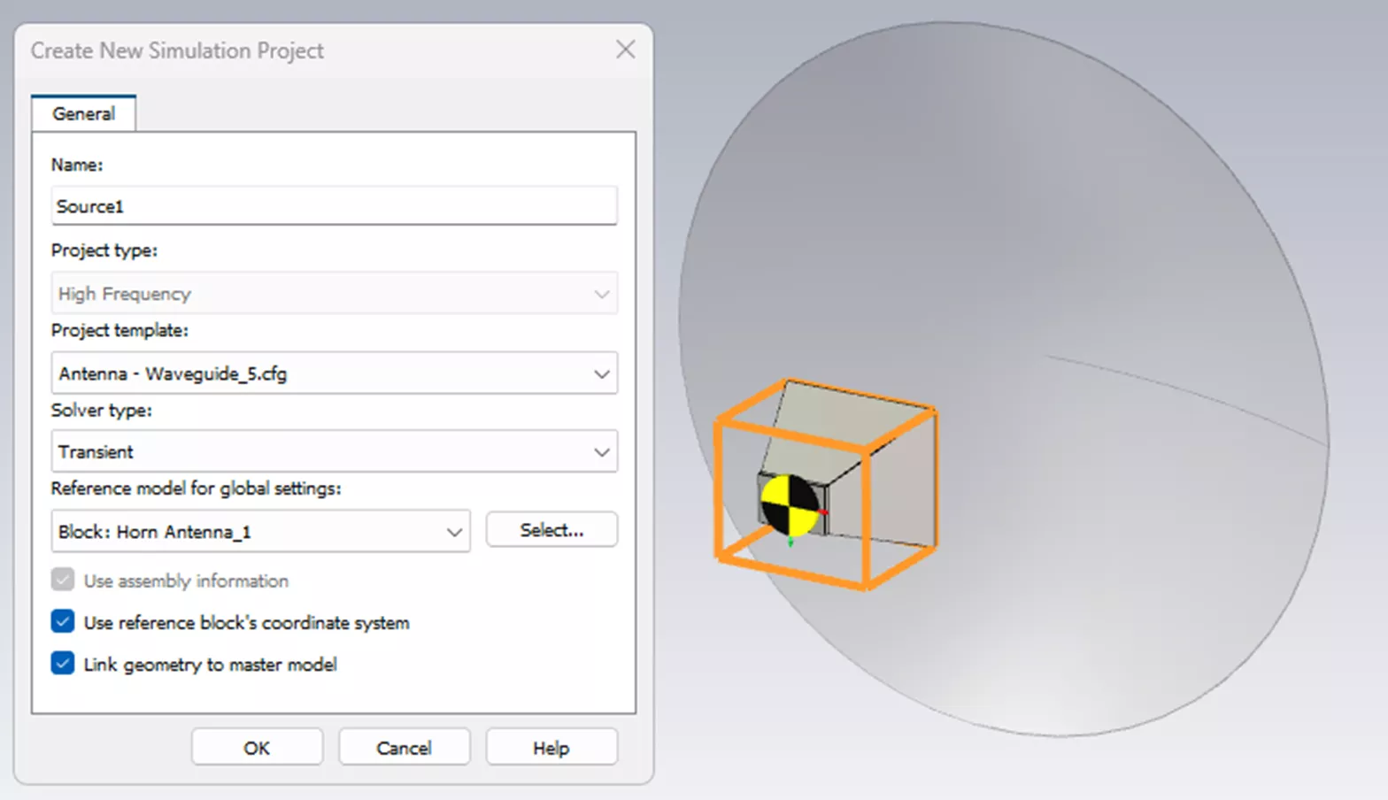
Figure 4 (c): Source project
Each simulation project is automatically created and can be accessed as a standard 3D project to analyze results for each step. To compare different scenarios of the assembly, multiple Hybrid Solver Tasks can be assigned with different task parameter settings such as coupling type, frequency range, and sub-domain solver. There are several solvers available for different applications such as time domain, frequency domain, asymptotic, integral, and TLM.
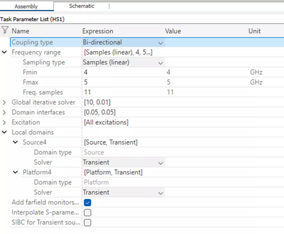
Figure 5: Task Parameter settings
After the simulation, the results associated with the Hybrid Solver Task are accessible directly from the Navigation Tree. You can easily compare the far-field results (figure 6(b)) for different coupling types and the selection of the sources (near-field or far-field) and optimize the design as needed. Hybrid Solver allows you to analyze S-parameters, antenna efficiencies, field distributions, surface current, far-field radiation patterns, and many more characteristics of the system.
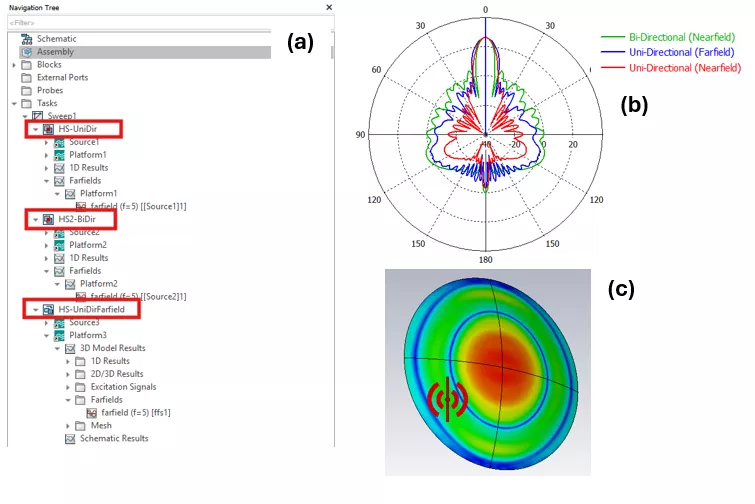
Figure 6: (a) Navigation Tree (b) Far-field results (c) Surface current distribution
Hybrid Solver is useful for simulating larger systems by decomposing the assembled system into individual domains. The main advantage of using the Hybrid Solver is that it significantly reduces the simulation time with a much lower system resource requirement compared to the brute force method while maintaining result accuracy.
Related Articles
Advancing Engineering Simplicity: SIMULIA’s New Unified Licensing Model
SIMULIA CST Studio Suite 2024 - What's New
Introducing the Unified License Model for CST Studio Suite
CST Studio Suite for Electronic Design
![]()
Get our wide array of technical resources delivered right to your inbox.
Unsubscribe at any time.