Abaqus FEA: Powerful Finite Element Modeling

The finite elements in “finite element analysis” (and how you create them) are fundamental. FEA users need to be able to easily create high-quality mesh patterns, and the algorithms behind the behavior of that mesh under load need to balance speed, accuracy, and capability to match the simulation’s intentions (whether that be a “quick and dirty” stiffness assessment or high-fidelity nonlinear stress analysis). 

A good and productive experience for the analyst comes down to the FEA tool’s capabilities with FE mesh and the meshing process. User-friendly, CAD-embedded FEA solutions, like SOLIDWORKS Simulation, are laser-focused on ease-of-use when accomplishing the most common FEA tasks, providing design guidance. A quick second-order tetramesh of a few parts is often all you need. 

But what about more specialized applications, increasing assembly size and interactions, or a “virtual prototyping” FEA use case? Then you may need Abaqus’ detailed mesh control, brick or prismatic element geometries, or specialized elements and element formulations. This article introduces some of what Abaqus can offer to help produce high-quality, purpose-driven FE models for better and faster analysis.

The Meshing Process: Geometry Discretization

Abaqus provides a variety of meshing methods and element geometries to suit any problem. The additional meshing techniques that Abaqus offers can potentially increase accuracy and reduce simulation solve time, but sometimes with limited applicability, based on component shape or the time the analyst has to produce a better mesh. Abaqus/CAE can also instantiate meshed parts the same way SOLIDWORKS can instantiate modeled parts.

Free Meshing

The simplest mesh technique is called  free meshing, as used in SOLIDWORKS Simulation. When meshing solid geometry, the surface is meshed first, then the volume is filled with solid elements. With free meshing, refinement control can be added to modify the final size of the elements in local areas by specifying the desired size for a portion of the geometry at the selected volumes, faces, edges, or vertices.

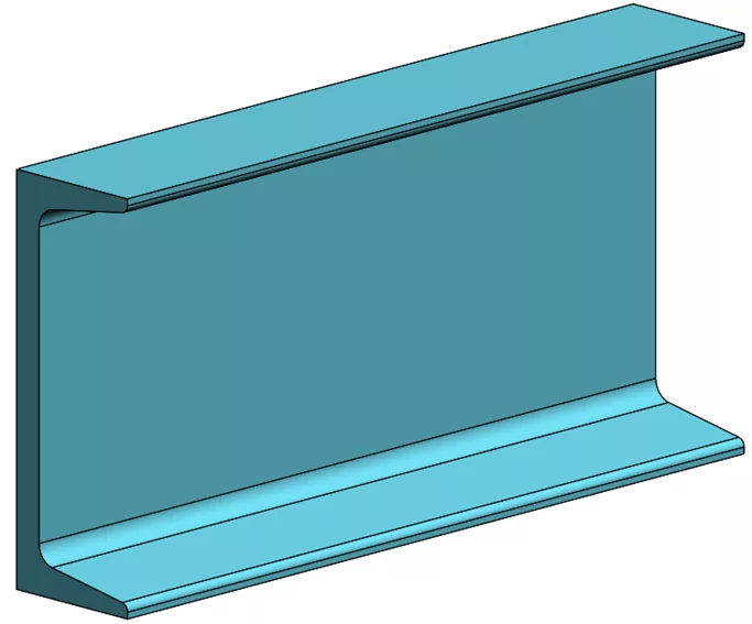
Channel beam section CAD

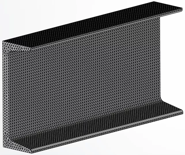
Channel beam section tetrameshed (48,800 elements)

Sweep Meshing

Abaqus is a tool for structural analysts and offers multiple methods to produce the desired mesh. Free meshing is one such method, but others offer benefits like greater refinement control or direct generation of specific element formulations that aren’t otherwise permitted with free meshing. One example is the sweep mesh technique, which is especially useful for common structural members produced as extruded parts. For comparison to free meshing, consider the simple rectangular beam.

Free meshing of the beam results in automatic generation of solid tetrahedral (tet) elements throughout, whereas a swept mesh will produce a uniform distribution of elements based on the 2D discretization of the starting face. In the image below a mixture of hexahedral (hex) and wedge/prism elements was produced.

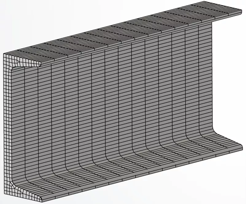
Channel beam section hexmeshed (2,600 elements)

The advantage realized with swept mesh is the ability to create multiple elements through the thickness of very thin parts without a high mesh count. The mesh of tets requires a total of 48,800 elements to get 3 elements across the web, whereas, for the HEX mesh, only 2,600 elements were required.

Even with the use of local mesh control available with tet meshing it is sometimes challenging to generate an adequate number of elements within the part volume without a high mesh count. A good mesh of hexahedral elements usually provides a solution of equivalent accuracy at less cost.

Partitioning

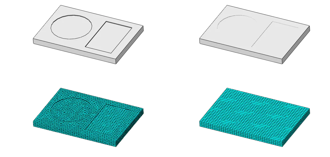
For some geometry, especially ones with bulky features and non-uniform cross sections (e.g., pressure vessel flanges and lifting lugs), free meshing is the best method to efficiently create the mesh. However, it is possible to use the partitioning tool in Abaqus to break the part into separate sections and mesh specific regions with different element types (shown below).

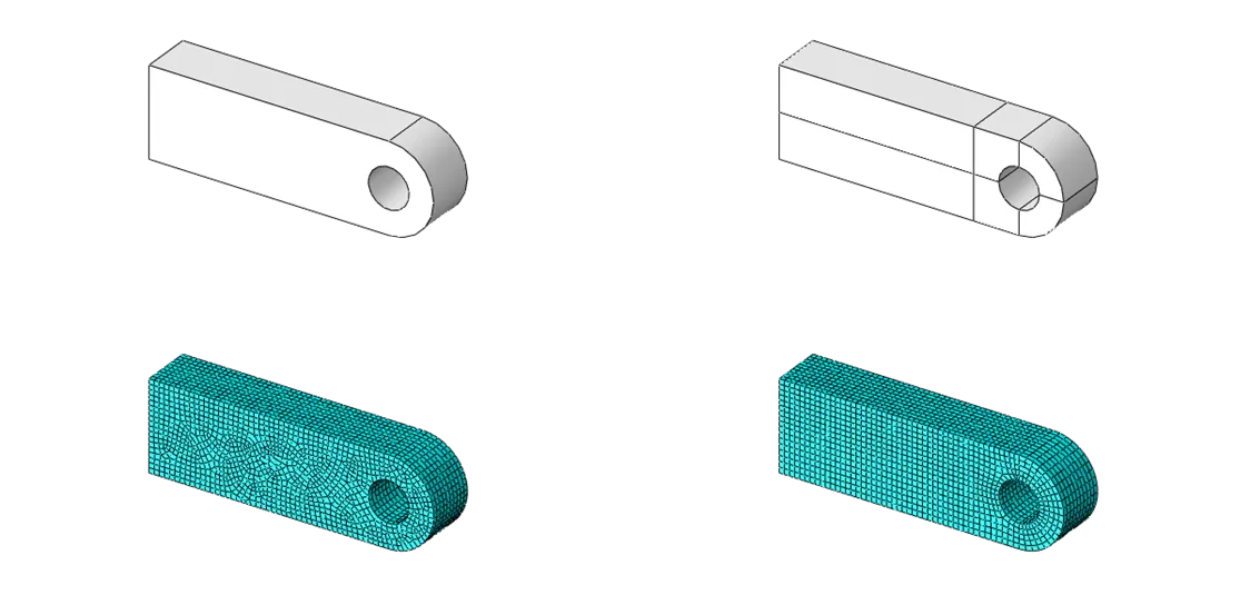
Abaqus/CAE partition; left (unpartitioned), right (partitioned)

Geometry Seeding

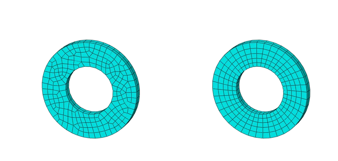
Meshing is further enhanced in Abaqus with geometry seeding . Effective use of seeding helps achieve uniform stress patterns that are critically important for accuracy where stress concentrations develop. Geometry seeding is a technique that allows for direct control of the element edge length in order to produce smooth transitions between geometric features. The desired mesh density in these areas is achieved by adding “seed” points along geometry edges where nodes are to be located. Below is an example of seeded edge control. The spacing between these seeds can be adjusted providing full control over the local mesh density.

Virtual Topology Constraints

For quicker mesh times and typically shortened solution times, Abaqus users can leverage virtual topology constraints, a functionality that removes small geometric features irrelevant to the analysis (shown below). By eliminating these small features, the meshing process becomes more efficient and the resulting mesh is simplified.

Mesh Associativity

Abaqus can enjoy CAD associativity with the use of  associative interfaces. With an associative interface for SOLIDWORKS, CATIA, or other CAD tools, the Abaqus/CAE preprocessor can pull directly from the original CAD rather than exported dumb solids. Analytical entities remain associated with the components and connections through CAD modifications, so the analyst doesn’t have to start from scratch with each iteration. The analyst can also modify CAD parameters from within Abaqus/CAE to quickly test hypothetical design alterations. These changes can be passed back to the original CAD if so desired.

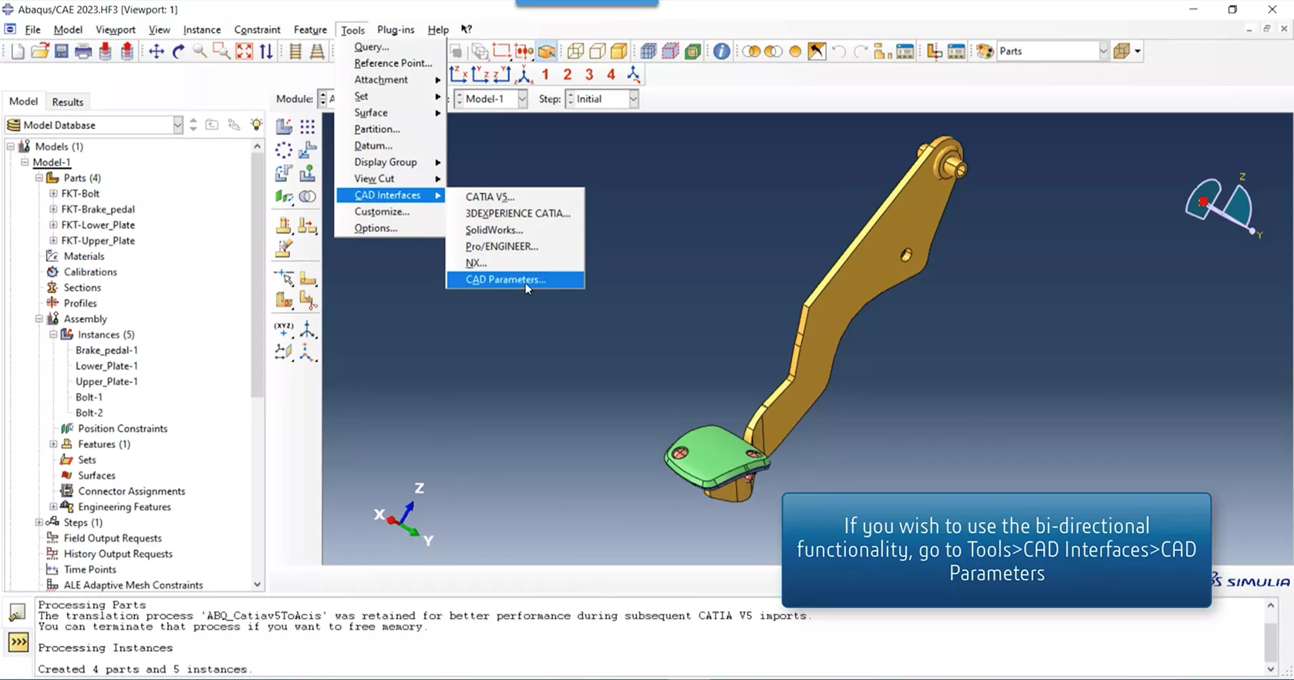
A user accesses CAD parameters from within Abaqus/CAE

Unassociated “Orphan” Mesh

Another advantage of Abaqus meshing capabilities is the ability to work directly with nodes and elements that are not associated with any CAD geometry. These “orphan meshes” may have been created in other pre-processors or even other finite element solvers. Abaqus/CAE allows users to edit the mesh by moving nodes, sweeping, splitting, or joining elements, defining boundary conditions, etc.

Mesh Adaptivity Techniques

In any finite element analysis, it is important to strike a balance between accuracy and efficiency. Stated another way, a good analysis presents the most accurate solution at the least cost. Most of the “cost” is controlled by the number of elements in the finite element model, which can be managed using mesh adaptivity techniques.  

Per the Abaqus User Guide: “The finite element discretization that results from suboptimal meshing of models can limit your ability to obtain adequate analysis results at a reasonable CPU cost. […] The adaptivity techniques available in Abaqus help optimize the mesh and, therefore, obtain quality solutions while controlling the cost of the analysis. The term “adaptivity” reflects the adaptive, or solution-dependent, processes that Abaqus uses to adapt the mesh to meet analysis goals. Three versions are offered and are usually selected based on their applicability to either accuracy or control of mesh distortion; their impact on mesh definitions, either through smoothing a single mesh or through generating multiple dissimilar meshes; and when [in the analysis process] adaptivity occurs.”

• Arbitrary Lagrangian-Eulerian (ALE) Adaptive Meshing
• Varying topology adaptive remeshing
• Mesh-to-mesh solution mapping

These techniques help improve the accuracy and efficiency of the simulation by dynamically adjusting the mesh resolution in regions of interest.

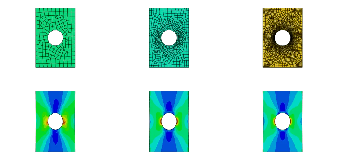
Abaqus/CAE adaptive meshing; iteration #1 (left), iteration #2 (center), iteration #3 (right)

Element Libraries: Type Selection for the Analysis Task

In addition to different element geometries (like tets vs. hexes), different element types can represent the same components using different numerical techniques, requiring potentially very different levels of setup and computation. For example, hex elements can represent the full volume of an extruded part, while infinitely thin quadrilateral shell elements can represent the thickness purely numerically with a thickness parameter, at greatly reduced computational requirements during the FE solve. In Abaqus, you will find an array of representational options for beams, connectors, rigid bodies, springs, and many more structural entities.

CAD Program Element Availability

As previously mentioned, the elements generated in CAD-based simulation tools, like SOLIDWORKS Simulation, are generated directly from the available geometry via free meshing. These programs produce solid (continuum), shell, and beam elements from the available solid, surface, and line geometry, respectively. As such, the elements are tied to the geometry. This is great functionality for the designer or engineer who produces quick design check simulations but may not meet the need for some applications.

Beyond the Basic Elements – The Abaqus Library

Analysts sometimes work on simulations that require more than the basic elements that CAD-based programs offer. Abaqus meets this need with a very full library of elements that can be combined however necessary in order to construct a computationally efficient finite element model.

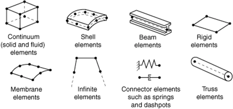
Commonly used Abaqus element families

Solid elements are commonly used to model bulky parts such as castings or forgings. Shell elements are more efficient for modeling thin parts such as sheet metal. Beam elements are efficient in modeling long, slender parts. For example, bolts are sometimes approximated using beam elements.

In terms of continuum and shell element shapes, Abaqus goes beyond the tetrahedral and triangular elements found in SOLIDWORKS. It includes additional element shapes, such as:

Quad/square: These shell elements provide improved accuracy and efficiency compared to their triangular siblings.

Hexahedral/brick: These elements have six faces and are suitable for representing volumes with more regular shapes, such as cubes or rectangular prisms. Hex elements are generally preferred due to their accuracy and efficiency.

Prism/wedge: Prism or wedge elements have a three-sided base and can be used to model structures with a more tapered or skewed geometry, such as pyramids or wedge-shaped components.

The image below shows some examples of different element shapes used to mesh the same cylindrical part within Abaqus CAE. Note how the hex elements on the left are able to capture the shape using the least number of nodes.

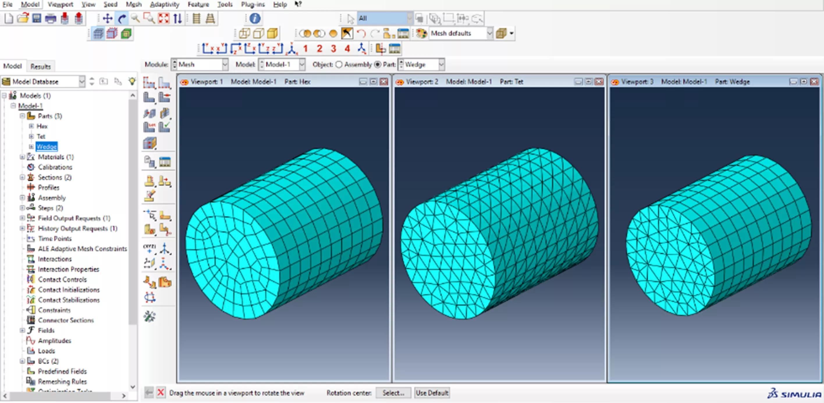
Abaqus/CAE solid elements; left (hex), center (tet), right (wedge)

Abaqus’ diverse library of element types finds applications across various domains and industries. Some lesser-known applications include:

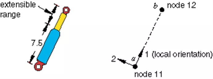
Connector elements: These versatile elements are used to attach two parts in some way. Sometimes connections are simple, such as two panels of sheet metal spot welded together or a door connected to a frame with a hinge. In other cases, the connection may impose more complicated kinematic constraints, such as constant velocity joints, which transmit constant spinning velocity between misaligned and moving shafts. In addition to imposing kinematic constraints, connections may include (nonlinear) force versus displacement (or velocity) behavior in their unconstrained relative motion components, such as a muscle force resisting the rotation of a knee joint in a crash-test occupant model.

Connector elements in Abaqus provide an easy and efficient way to model these and many other types of physical mechanisms whose geometry is discrete (i.e., node-to-node), yet the kinematic and kinetic relationships describing the connection are complex.

Discrete particle elements: The discrete element method is useful for modeling discrete particles or granular materials to simulate their interaction with containers. Thanks to the powerful Abaqus General Contact capability, these elements may interact with each other and any other elements in the model. An example of granular media mixing in a drum mixer is shown below.

Mixing of granular media in a drum mixer

Special-purpose elements: Abaqus includes elements dedicated to specific applications, such as acoustics, cohesive elements for modeling fracture or delamination, hydrostatic elements for simulating fluid behavior, and more. An example of post-buckling and growth of delamination in a composite panel is shown below.

Post buckling and growth of delamination in a composite panel -By providing a wide range of element types and shapes, Abaqus offers users the flexibility to accurately model and analyze diverse structures and phenomena in their simulations

Element Families: Order, Integration Method, Section Control

Whereas CAD the SOLIDWORKS Simulation program offers first and second-order element formulations, Abaqus offers additional element characterizations that allow users to tailor their analysis to specific requirements, ensuring accurate and reliable results. These options enhance the versatility of the software and enable users to tackle a wide range of problems, from standard structural analysis to complex phenomena involving large deformations, fluid-structure interaction, or material failure. They also allow the user to fine-tune speed vs. accuracy where it matters to them.

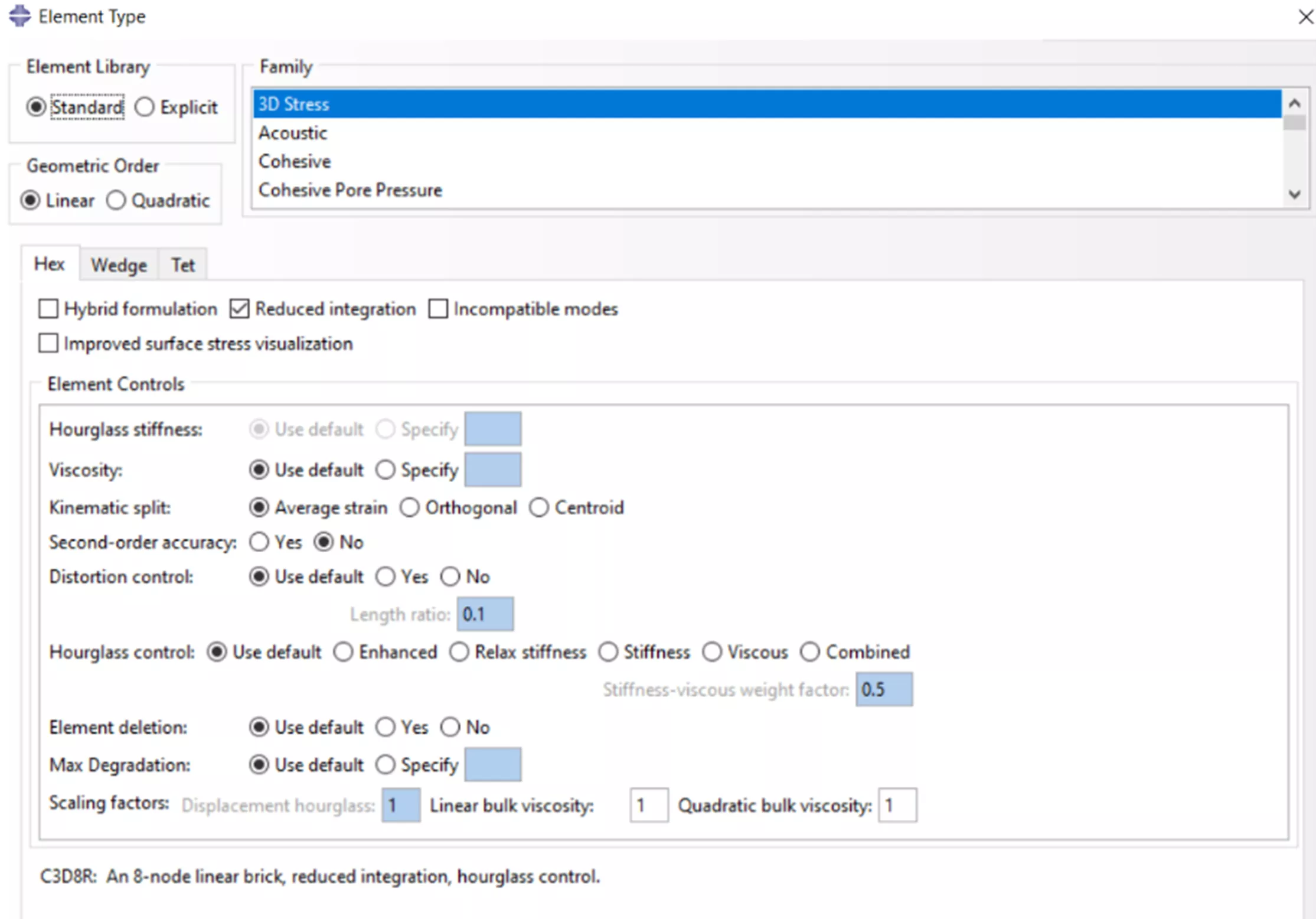
Abaqus/CAE solid element controls

These characterizations allow for further customization and control over the element behavior and integration scheme:

• 2nd-order elements: The element formulation can be adjusted to meet specific modeling requirements or to capture phenomena more accurately.
• Formulation options: Lagrangian and Eulerian formulations are available. The Lagrangian formulation is commonly used for most solid and structural analyses, while the Eulerian formulation is suitable for problems involving large deformations, fluid-structure interaction, or material separation. Additionally, Abaqus provides a continuum shell formulation specifically designed for thin structures.
• Integration options: Users can choose between full integration and reduced integration schemes for elements. Full integration offers more accurate results by integrating the material properties and governing equations over the entire element volume. Reduced integration, on the other hand, provides computational efficiency by integrating over a reduced number of integration points, sacrificing some accuracy for faster computations.
• Section control: Various options are available in some element types. These include preventing hourglass modes, limiting element distortion, and accounting for material damage or failure during the analysis. These controls enhance the stability and accuracy of the analysis by mitigating issues related to element behavior.

Beyond Structural Simulations

Abaqus FEA is a workhorse when it comes to structural simulations, but its meshing and element functionality goes beyond structural, offering elements to serve other physics as well, such as Eulerian elements with fluid-like behavior. This flexibility allows users to model and simulate fluid dynamics, multiphysics phenomena, and other non-structural scenarios using the Abaqus software.

Hot forging simulation: CEL thermal stress simulation with contact interactions

In addition, Abaqus provides tools for resolving common mesh difficulties encountered in complex geometries. These tools assist in geometry repair, ensuring that the mesh accurately represents the intended design. By addressing these challenges, users can achieve reliable analysis results and accurate representation of the geometry.

Conclusion

CAD-based simulation programs such as SOLIDWORKS are well-suited for basic structural and thermal analysis and typically have a user-friendly interface that provides unparalleled efficiency with a specific selection of popular FEA processes. But when you brush up against the limitations or need to step outside the box, Abaqus offers a great variety of expanded capabilities in the area of the finite element model. Its wider range of meshing techniques and algorithms enables complex simulations, more complex assembly interactions, and faster computation of accurate model behavior.

Read our Abaqus buying guide or reach out to one of our GoEngineer simulation experts to find the right tool for you! If you’re not ready to use Abaqus yourself, you can still take full advantage of its benefits through FEA consulting from GoEngineer.

Related Articles

Abaqus Solvers: Empowering Engineers in Every FEA Scenario

FEA and CFD Analysis Software: What to Know Before You Buy

SOLIDWORKS Simulation vs Abaqus: When Should You Upgrade?

The Ultimate Guide to Abaqus Computing

8 Ways Working with an FEA Consultant Improves Your Bottom Line

VIEW ALL ABAQUS ARTICLES