Understanding Abaqus General Contact

For many analysts, the term ‘contact’ in finite element analysis (FEA) evokes memories of complex setups, convergence headaches, and often, compromises in accuracy. Traditionally, modeling contact via the contact pair approach has been notorious for its demanding requirements in terms of model preparation. Not only was the user responsible for manually choosing the surfaces to be in contact, but it also required the user to build the entire contact formulation; so, specifying the surface assignment, the contact tracking approach, as well as the surface discretization method.

Recognizing these challenges, Abaqus introduced a groundbreaking solution to overcome the limitations inherent to the traditional contact pair approach: General Contact. This highly sophisticated method for modeling contact and interaction problems is distinct from the contact pair method. By using powerful tracking algorithms, General Contact can efficiently enforce and simulate contact conditions, ensuring accurate simulation outcomes. For a SOLIDWORKS Simulation user, the main advantage of using contact in Abaqus (or in 3DEXPERIENCE STRUCTURAL, which uses the Abaqus solver) is improved robustness. There are also some special features and conveniences to help define contact, which may make it easier to run contact on large assemblies. In this article, we take a deeper dive into Abaqus’ General Contact.

Robustness of General Contact

Abaqus/Explicit

General Contact in Abaqus starts with prescribing the contact domain via an automatic, all-inclusive contact surface. This all-inclusive surface includes all element-based surface facets, all analytical rigid surfaces, and – in the case of Abaqus/Explicit – surfaces on all Eulerian materials (typically used for fluid-structure interactions). General Contact uses sophisticated methods to ensure that proper contact conditions are enforced efficiently. In Abaqus/Explicit, it generates contact forces to resist node-into-face, node-into-analytical rigid surface, and edge-to-edge contact penetration across the all-inclusive surface, thereby providing a comprehensive solution for enforcing contact in a wide range of simulation scenarios without the need for complex contact definition procedures.

When special cases require it, the general contact algorithm can be used in conjunction with the contact pair algorithm. It is available for two-dimensional, axisymmetric, and three-dimensional surfaces, but can be used only in mechanical finite-sliding contact analyses. It does not support kinematic constraint enforcement, but instead uses the penalty method to enforce contact constraints.

Abaqus/Standard

The general contact algorithm in Abaqus/Standard dynamically detects and manages various contact types—surface-to-surface, edge-to-surface, edge-to-edge, and vertex-to-surface—throughout the analysis, enhancing its capability for complex interactions. Utilizing a finite-sliding tracking approach, it's especially effective for three-dimensional models and is the sole method for two-dimensional and axisymmetric models. This algorithm is impressive at adapting to changes, seamlessly transitioning between contact formulations as the analysis evolves.

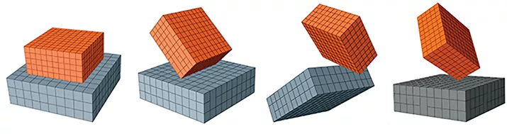
Figure 1: Contact scenario types for two blocks

For instance, in a snap-fit simulation, it might initially prioritize edge-to-surface contact, then smoothly shift to surface-to-surface contact as the engagement area expands. This adaptive approach ensures accurate application of contact constraints and avoids numerical issues, making Abaqus/Standard robust for a wide range of simulation scenarios.

To illustrate the robustness of the general contact algorithm, consider a simulation involving a rubber cuboid sliding around the perimeter surface of a larger rubber cuboid. At the beginning of the analysis, as the smaller cuboid approaches the larger one, surface-to-surface contact is established. The algorithm then detects contact changes as the cuboid reaches a feature edge of the larger one and implements an edge-to-surface contact formulation. This on-the-fly approach significantly enhances the algorithm's robustness and reliability for handling any changes in contact.

Figure 2: Rubber cuboid sliding around another rubber cuboid

Convenience of General Contact

General Contact, whether it be in Abaqus/Standard or Abaqus/Explicit, allows the user to define the contact domain with flexibility and precision. This includes specifying general contact inclusions to identify potential interaction regions and contact exclusions to omit certain interactions, ensuring accurate and efficient analysis.

For both Abaqus/Standard and Abaqus/Explicit, the general contact domain can be defined using an “automatic” option, incorporating all exterior element faces, edges, and analytical rigid surfaces. This default, all-inclusive surface simplifies the setup by automatically considering all possible node-to-face, edge-to-edge, and self-contact interactions, without the need for manual specification of individual contact pairs. Users can refine the contact domain by specifying specific surfaces or materials to be included or excluded, and add individual property assignments. Users can further refine the general contact definition by tweaking it throughout the analysis, activating and deactivating certain surfaces to be part of the contact domain as necessary. The process is seamless and convenient, yet it gives the analyst the ability to tweak and fine-tune the contact domain as needed.

The setup process is designed to apply contact inclusions first, followed by exclusions, with the latter taking precedence. This hierarchical approach allows for precise control over the contact conditions considered in the simulation, facilitating the modeling of complex assemblies and interactions with ease. Both Abaqus/Standard and Abaqus/Explicit automatically generate contact exclusions in certain situations, such as when interactions are defined using contact pairs or surface-based tie constraints, to prevent redundant enforcement of interaction constraints.

The following example of a Jenga Tower analysis illustrates the convenience that the general contact algorithm brings when dealing with a large number of parts.

Consider this Jenga tower, made up of 18 layers in total, with three pieces of Jenga in each layer. This gives a total of 54 pieces. The chaotic and unpredictable nature of this analysis can be seen in the animation below. It’s for this very reason that the general contact algorithm is used, allowing for the consideration of all faces that are initially in contact as well as those that may come into contact later in the analysis.

If this analysis were to be done without using the general contact algorithm, manual selection of contact faces would have to be done to achieve a comparable result. For the sake of explanation, we will compute the number of contact faces the analyst will have to define, manually. Each piece of Jenga has 6 faces, and to be on the safe side, we will assume that it is possible for each face to come into contact with the faces of all other 53 pieces. This means that each piece of Jenga carries a total of

We still have to account for duplicates, meaning that face A touching face B is the same as face B touching face A, so the number of faces needs to be divided by 2. And, to account for all other 53 pieces of Jenga with each of their faces, the total number of contact pairs that the analyst would have to account for is

51516 is a ridiculously high number for such an analysis. And so, one can start to appreciate the robustness and convenience of the general contact algorithm.

Figure 3: Animation of Jenga Tower analysis

Special Features in General Contact

Fluid Pressure Penetration

A pressure penetration load allows for the simulation of the pressure of a fluid seeping between surfaces involved in contact. The pressure load may deform the components, potentially opening a small gap which exposes additional surface area to the pressure. This is an extremely useful feature for sealing an analysis, and it runs very efficiently in Abaqus since it does not require modeling the fluid itself. The bodies involved may both be deformable, or one can be rigid, as occurs when a soft gasket is used as a seal between stiffer structures.

An example provided in the manual involves fluid pressure-penetration loading of an O-ring seal in a pipe connection. This simulation models the fluid pressure loads as either distributed surface loads or pairwise pressure loads, highlighting the wetted surface evolution based on contact conditions. It showcases the application of fluid pressure on surfaces that undergo significant deformation, such as the self-contact of rubber, employing both explicit and implicit dynamic procedures to approximate quasi-static conditions.

Figure 4: Evolution of fluid pressure

Approximation of Threaded Contact

The localized load distribution in threaded joints may be approximated without meshing the threads. The meshed parts typically have cylindrical surfaces at the interface with this approach. This capability adjusts contact normal directions to be normal to faces of reference threads. This added level of detail compared to simply bonding the threaded surfaces can be important in bolted joint analysis.

The below screenshot shows the contact normal for the two threaded parts, the bolt (in green) and the nut (in beige).

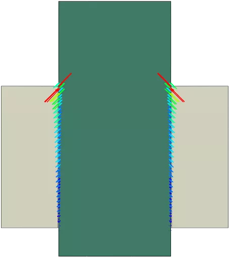
Figure 5: Contact normals of "threaded" parts

Precise Values of Clearance and Interference

Precise values of clearance or overclosure may be specified and modified independent of the geometry or mesh accuracy. For example, it is not necessary to model a 20 μm gap between components; the gap can be modeled line-on-line and specify that the solver should treat this as 20 μm This also makes clearance or interference sensitivity studies very efficient to setup and run without the need to re-mesh any components.

Surface Erosion

Surface erosion is important to consider when dealing with material failure. This is facilitated by the general contact algorithm when modeling surface erosion by utilizing element-based surfaces, thus allowing us to simulate how surfaces evolve in response to material failure. When defining surfaces for erosion, it’s best to use element-based surfaces for the eroding body. This helps in accurately capturing the changing contact domain as the material degrades and fails. Not only does this approach simplify the modeling process, but it also enhances efficiency by reducing memory usage compared to using interior surfaces.

Erosion modeling is particularly useful as it dynamically updates the contact domain to reflect the removal of failed elements, thereby adjusting the active contact faces and edges. This dynamic update ensures that the simulation remains accurate throughout the analysis, mirroring real-world material behavior under stress or impact.

Additionally, the choice to include nodes in the contact domain after surrounding elements have failed can be controlled, offering flexibility in simulating the aftermath of material failure and its impact on structural integrity.

To illustrate the application of surface erosion, consider the simulation of an eroding cylinder projectile impacting an armor plate at high velocity. This example uses General Contact to model the interaction between the projectile and the plate, both of which are subject to material failure.

The scenario simulates the oblique impact at 2000 m/s, with the material for both bodies defined to include failure models that account for progressive damage. As the elements fail due to the impact, they are removed from the simulation, and the contact surfaces adapt to reflect the newly exposed surfaces of the remaining elements.

This approach not only captures the immediate effects of the impact but also the subsequent changes in the contact domain as the material erodes. Such detailed simulation helps in understanding the complex behavior of materials under extreme conditions and demonstrates the power of the general contact algorithm in handling sophisticated contact and failure scenarios.

Figure 6: Eroding cylinder projectile impacting an armor plate

Conclusion

In conclusion, Abaqus offers a comprehensive and sophisticated general contact algorithm that simplifies the modeling of contact and interaction problems, ensuring accurate simulation results. The ability to efficiently simulate contact conditions, from surface-to-surface to edge-to-edge contact interactions, enhances the robustness of simulations. This, combined with the convenience and ease of setting up General Contact, makes this contact algorithm very attractive and desirable for SOLIDWORKS Simulation users.

The benefits of Abaqus contact can be very material. General Contact opens the doors to innovation by enabling the kind of detailed contact analysis that was previously unattainable. For example, exploring the full potential of Abaqus’s general contact algorithm unveils opportunities in fields like biomechanics, for simulating joint or dental implant dynamics, aerospace, for enhancing landing gear and turbine interactions, and consumer goods, for high-energy impact improving durability. Such advanced FEA capabilities encourage engineers to venture into new simulation territories, pushing product development and material science into the future.

Read our Abaqus buying guide or reach out to one of our GoEngineer simulation experts to find the right FEA tool for you! If you’re not ready to use Abaqus yourself, you can still take full advantage of its benefits through FEA consulting from GoEngineer.

Related Articles

Understanding Abaqus Material Behavior

FEA Critical Speed Analysis & Rotor Dynamics

Abaqus FEA: Powerful Finite Element Modeling

Abaqus Solvers: Empowering Engineers in Every FEA Scenario

FEA and CFD Analysis Software: What to Know Before You Buy

VIEW ALL ABAQUS ARTICLES

Contributing Author: Shaun Bentley